How Zone System Works: A Conceptual and Technical Sketch part II
(This article is part II in a series. Reading part I is essential as it establishes the scientific basis of tone reproduction. My intention in this series is to disseminate accurate information about sensitometry and Zone System for the photographic community.)
4.0 Image Processing
In the previous article I explained the general technical basis of sensitometry and Zone System and its benefits to the photographer. Simply, in a well-controlled photographic system the artist can satisfactorily correlate the appearance of tonality in a scene and the final image. However, what remains is to address the middle step of Processing which brings the scene and final image into alignment.

The previous article addressed the beginning and end of this chain. This article focuses on Processing, the middle block.
I will begin with explaining the analog process for three reasons. First, sensitometry started with analog so this medium is the most studied and documented. Second, the analog process has very rigid controls which give us a straighter arrow to follow. Finally, there is a level of transparency to the process (all puns intended) compared to digital steps in a computer which hide some of the signal processing.
4.1 Thinking Backwards
For all photographic materials the most important limit to tonality are the limits of the print, projector or monitor. This statement is so crucial to the correct application of sensitometry it is worth reiterating - the medium of the final display dictates how to expose and process the negative. This means that the tonal rendering of the photographic paper determines how to expose and develop the film. The flexibility of changing a digital file in a computer often cloaks the fact that the electronic display, whether a monitor or projector, also determines how we should be exposing and processing the digital image. Even though we learn about the photographic process beginning with the camera and ending with the print - the analysis of tone reproduction is viewed backwards.

Diagram 4.0 - We learn photography as a process from scene to print. However, the science of sensitometry looks backwards through each link in the chain in order to understand tonal rendering at each subsequent step in the process.
In order to really appreciate the quantitative and qualitative changes in tonality in the processing phase of an image it is necessary to look at the sensitometric graphs that accompany this step.
4.2 The Sensitometry Graph and Transfer of Tonality
There is a power in graphs - they easily reveal relationships between each step in a process. Let me take a moment to give a brief explanation of sensitometry graphs for analog and digital materials before exploring how these relate to the print paper and computer monitor.
The x-axis of the graph is the incoming light from a scene. For a sensitometry analysis the scene consists of a range of discrete steps of tonality (such as a grayscale chart like the Kodak Q-14) or a series of images of an underexposed and overexposed graycard. The scale of the x-axis is typically shown in steps of log exposure (log(H) with H=lux x seconds) where each step of 0.3 is one stop in change of the illumination. More recently it is common to show the x-axis in camera stops. While camera stops are more familiar to a practicing photographer there must be an indication of the proper exposure point a scene. In the graphs for Kodak’s Vision 3 motion picture films correct exposure at the manufacturer’s EI is indicated by a 0.
Against the change in intensity of light from a scene one can measure and plot the amount of signal captured by the medium . Film records light as silver density (or dye in the case of the colored film) so the y-axis on a film graph is density. All film graphs use a logarithmic scale where each step of 0.3 is one stop change in density. (Neutral Density filters use the same scale!) Digital files store the signal as a string of bits and the length of this string is the bit-depth. For digital sensitometry graphs the y-axis can be either bit depth, or a percentage of bit-depth. The slope of the straight line portion of the graph is the contrast. The steeper the slope of the curve, the more contrasty the image and vice versa.

Diagram 4.1 - At top is a generic sensitometry diagram labeled with key terms. Both analog and digital share the same x-axis scale. However, the y-axis is different since film records the image as density, and digital records in terms of code values.
Obviously, we don’t display the camera negative, nor can we see the stored digital file. So the captured information is made visible by moving the recorded signal to a display - photographic paper for analog, or an electronic monitor in the case of digital. We can analyze this transfer of tonal information by mapping the curve from the capture medium to a curve for the display medium. In diagram 4.2 I show this transfer from the negative to the steep curve of the paper.
By analyzing the entire photographic chain through sensitometry graphs the need to match the limits of our materials becomes imperative. If we have two curves to work with, the curve of the negative and that of the print, why do ZS photographers work so hard on exposing and developing the negative? In fact, you may have heard their adage “expose for shadows and develop for highlights.” The reason is that the curve of the print paper is very steep, and any small change in printing and developing time has a large impact on the final tonality. It is simply more practical to work with one grade of paper, calibrate the negative to that specific grade, and then work within the parameters of dodging and burning only. Of course, we do have the option to switch grades of paper if we need an image to have more or less contrast. But simply, the flexibility of the negative in processing and exposing is just so much greater and easier to control.
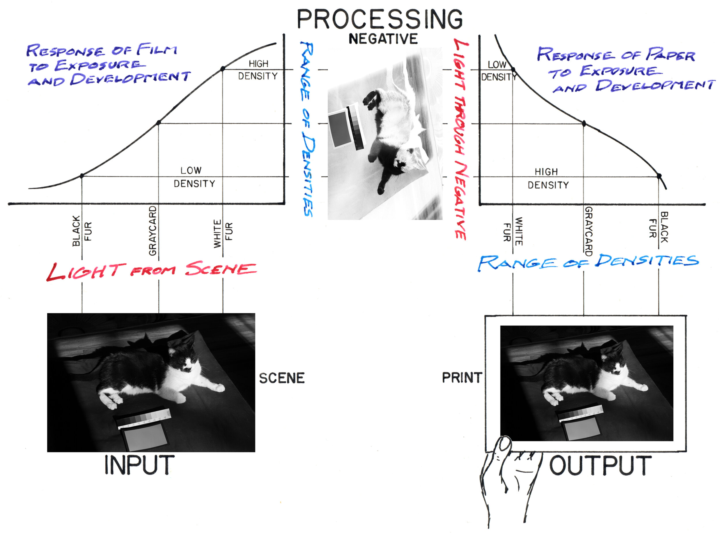
Diagram 4.2 - Follow this graphic from Input in the lower left clockwise through to the Output. One can understand for film / print materials how the light from the scene is recorded as density on the developed negative. Then, light is transmitted through the negative to expose and develop a print. Provided a system is well calibrated by Zone System techniques the photographer can have excellent control over how the tones from the scene are rendered in the final print.
So how to control tonality? Well, it involves spending time testing materials with calibration charts – standardizing one’s post-process – and then spending a period of time light metering and taking notes in the field. In a next post I will spell out a step-by-step guide of how I calibrated my film/paper combination. For now I want to demonstrate the generic process of control within a calibrated film and digital system.
5.0 Analog Image Control
In the analog image chain we rely on altering contrast and tonality by:
Film Development Time – Determines the contrast of the captured information from the scene.
Paper Grade – Typically ZS practitioners calibrate for paper grades 2 or 3. This allows for the use of grade 1 if a lower contrast is required, and grades 4 and 5 if the image needs more contrast. However, we expose and develop our negatives so as not to need these extreme ranges of paper grades.
Dodging/Burning – Localized changes in tone by blocking the light from the enlarger (dodging) to make that area lighter or exposing it for longer to make it darker (burning).
While one could rely on grades of paper and dodging/burning alone it is far from ideal. I have printed difficult negatives and the range of physical motions I have to make, the time in which they must be performed becomes a narrow tight rope leading to many rejected prints and problems with reproducibility. Better to have an optima negative so that tones fall in a close to desired way. When this occurs all further tone adjustments through dodging and burning are much easier.
So how does one control their curve of the negative? By development time – a longer development time (push processing) raises the contrast and a shorter development time (pull processing) lowers the contrast.

Diagram 5.1 - The sensitometry curves from Tri-X in T-max developer. Notice that as the development time increases the curves become increasingly steeper. From Kodak Technical Publication F-4017, February 2016.
There is an important ramification to changing the developing time, which is that the recorded density from the scene is moved to a less ideal part of the dynamic range of the negative. If one does not decrease exposure in response to a longer developing time the highlights can be too “bulletproof” to print and an increase in grain across the image. To compensate we change the EI of the film to a higher number, as if the film is more sensitive to light. For example, in my tests with Agfapan APX400 in PMK I discovered that 12 minutes of developing time gave me an EI of 100. However, increasing the developing time to 16 minutes required an EI of 125 to keep Zone II in the lower part of the curve.
Conversely, the image loses shadow detail if there is no exposure compensation for the shorter developing time. Therefore, we lower the EI as if the film is less sensitive to light. Looking at my Agfapan APX400 notes the change from a 12 minute developing time to an 8 minute developing time resulted in an EI of 80. Some of you may be thinking that such little change in EI to developing times is not a big deal. However, this is just the case of my materials and these relationships can be dramatically different depending on the developer and film combination one chooses.
Moving further backward through our analysis we can also determine the range of light in a scene that is held by our film/film development/paper combination. I found that within my system, (grade 2 paper in Sprint Quicksilver developer, APX400 with an EI of 100 and developed in PMK for 12 minutes) that I obtained a 7 stop range of light in my scene. This allowed me to go out in the field and take spot meter readings reliably knowing any object 3 1/2 stops over and 3 1/2 stops under proper exposure were outside the limits of tonality rendered with detail. You will also notice that this 12 minute development time is a good normal development time that places an object 3 1/2 stops under middle gray in Zone II, and an object 3 1/2 stops over middle gray in Zone VIII.
Two quick points – 1) Remember, the negative records more than the narrow window of 7 stops. What we are accomplishing through this sensitometry analysis is how to optimize our system so light in our scene is easily rendered as the same Zone in the print through manipulation of development time and EI alone. This gives us an easier image to finesse into our desired intention. 2) This 7-stop range are tones with detail. We know the scene will have objects beyond these tones that are black and white.
Armed with my 7-stop range I can spot meter objects in my scene to see whether they fall with the ideal recorded density of my negative. So what do I do if my subject has a greater range than this “normal” developing time? Well, let’s look at our cat picture again.
If spotmeter readings of our subject have these values…

Diagram 5.2 - These are possible spot metered values for a high contrast object. Notice that the white and black fur that we want rendered with detail are four stops over and four stops underexposed.
…I would pull process in order to lower the contrast on my negative. This development allows the critical highlight and shadow details to fit within the limits of the paper.

Diagram 5.3 - This is the transfer quadrant for a scene that is too contrasty. The cat’s white fur which we want in Zone VIII is in Zone IX and the black fur which should be in Zone II is in Zone I. Pull Processing (sometimes called Contraction Development) of the film places all the tones back into their proper location.
What if my scene is too low in contrast? Let’s say I get these spot meter readings…

Diagram 5.4 - In this situation the subject’s white fur is only metering two stops above middle gray and the black fur is only two stops under. The cat looks low in contrast and we want to place the white fur back into Zone VIII and the black fur into Zone II.
…I would push my film to increase its contrast in order to fit the paper.

Diagram 5.5 - This is the transfer quadrant for a scene that is low contrast. The cat’s white fur which we want in Zone VIII is in Zone VII and the black fur which should be in Zone II is in Zone III. Push Processing (sometimes called Expansion Development) the film places all the tones back into their proper location.
Keep in mind, these examples are merely to illustrate how to make an image of the cat with the fur in the appropriate zone for ‘how it appears to the eye.’ However, recognizing how development time controls tonality opens a world of aesthetic controls to the artist and their intended vision.
The previous examples are simplified by relating the same light meter readings to film development time. However, the decision to change development time requires the photographer adjust the Exposure Index of the film. By lining up our three development curves (normal, pull, and push) on one graph the necessity of altering the exposure time becomes apparent.

Diagram 5.6 - This is idealized to illustrate basic concepts. For a real world diagram just look at 5.1 above with the different development curves for Tri-X.
Notice that as the development time is changed the point where Zone II begins is displaced horizontally. Since the x-axis is the scale of exposure the distance these points move in stops can be used to calculate the change in Exposure Index. This point is also called the speed point in sensitometry since it is used to calculate the speed rating of the film. In our example the speed point is moving one stop on the Log Exposure scale so the Exposure Index is changed by the same amount. If my film is 200ei with normal development and a spotmeter reads the graycard as f/4 then that is the aperture I will set my lens. However, if I wanted to push the film I would need to set my aperture to an f/5.6 to compensate for the longer developing time. If I wanted to pull my film I would set my lens to an f/2.8 to compensate for the shorter developing time. I could also adjust my shutter speed instead of aperture if I did not want my Depth of Field to change and my subject remained static.
If you have ever heard the famous adage “expose for shadows, develop for highlights” you can begin to unpack the remarkable truth this statement encapsulates. That is, your choice of EI places your shadow details to a point on the curve that keeps the detail of shadows intact, and then the choice of development time sets the slope of the curve to position the highlights. The calibration tests I explain in the next post will give a working example from my own tests. However, in sensitometry graphs we can see this interrelated dance of EI and development times.
I should make two more important points for clarity:
First, I cannot stress enough that the process of calibrating a film/film development time/paper/paper developer and the temperature and agitation techniques is a total system. Once one starts changing different parts of each control than different tonal results occur. The analog photo chain requires a high degree of discipline.
Second, the control of the curve of the negative is made by the photographer at the moment of exposure. The act of determining exposure and developing time in the field dictates the darkroom process. This can be changed, but only by so much. This is why ZS emphasizes the skills of memory, calibration, rigor, and practice.
6.0 DIGITAL
An understanding of analog tone control is easily translated to the digital image making process. The greatest difference lies in the fact that the “developing” of a digital image is now in a computer where a myriad of controls await. In fact, I think adjusting the image in a photo editing software is so easy that many don’t realize they are undertaking similar steps as with film – setting the brightness and contrast of the image curve to fit the limits of the display – now a computer monitor.
Your monitor is set to an EOTF, or electro-optical transfer function. This is a conversion function to translate from electronic code values to an intensity of light. The EOTF is the equivalent to the sensitometry curve of photographic paper. Computers commonly use a gamma of 2.2 as graphed below. I chose to graph the y-axis on two different scales - an exponential scale and a logarithmic scale. On the logarithmic scale the 2.2 gamma reveals an S-curve shape. This is more analogous to film/paper curves because the y-axis is showing each step on the graph as a change in one stop - so each step is a doubling of the output of light from the monitor.

Diagram 6.1 - On the left is a gamma of 2.2, the conventional gamma for sRGB and Rec709. The x-axis are 8-bit code values and the y-axis is the luminance of the monitor if calibrated properly. On the right is the same data, but with a logarithmic y-axis scale. Each step on this scale is a whole stop change in luminance. Notice the emergence of the S-shaped curve as well as the steepness of the curve. Notice that currently the sRGB and Rec709 standard only displays around 8 stops of dynamic range.
Notice that the monitor also has a steep curve similar to that of a photographic paper. For our cat example to display correctly we need to adjust the curve of the captured image to make it fit within the limits of the monitor. To accomplish this our ‘developing’ is replaced by the use of the curve tool or wheels. (Now you understand why this tool is called a ‘curve’ tool - it derives its principles from sensitometry!) However, the laborious process of calibrating film is replaced by simple computer adjustments while you view the changes to the image in real time.

Diagram 6.2 - Notice that this is very similar to the analog tone transfer diagram but with a few alterations. The image is captured in a file format that is then corrected in a computer. For this example I selected a RAW capture that has its metadata and a curve applied in the computer.

Diagram 6.3 - Here is a screenshot from adjustments to the same image in a photo editing software. While the curve tool is inspired by the sensitometry characteristic curve, it doesn’t actually map the tonal rendering of the image. Instead, it just provides a straight line tool for further adjustment to whatever data is there. Here I applied a ‘medium contrast’ curve and then proceeded to nudge the midtones higher. If this image was analog I would have developed the negative for the same desired contrast. Next, I would have dodged up midtone areas in the image. So in the computer you are using the curve or wheel tools as both your ‘developing’ and ‘dodging & burning.’
The possibilities in image editing in a computer are vast and displayed immediately for our assessment. I think this is where the chain of tone reproduction is so seamless one could be using a “light” form of ZS without knowing it. After all, you are mapping the tones of a scene into a desired place by using one’s visual memory and visual system as the comparison. What many don’t realize is that the tone reproduction process for film and digital share the same principles. No matter the format you begin by viewing a scene with the limited range of your eye, captured it with a photographic system with a large dynamic range, but are now compressing the limits back down to limits of your eye in the final display.
7.0 Tying it All Together
Armed with a knowledge of how we see tonality, and how our final display depicts tonality, we are empowered to transform the curves of our capture medium to bring our vision and the final image into alignment. More importantly, we can use this information in order to interpret light meter readings of a scene. This ensures that objects are reproduced as intended in printing and are far away from the limits of the dynamic range.
There are perhaps two lingering questions: 1) Why is the S-shaped curve so predominant?
Sensitometry studies on people have shown this to be the most characteristically pleasing mapping of tonality. On a pure technical level a straight line with a slope of 1 would be ideal, but we are making these images for people’s enjoyment. The reason for the slightly crushed toe of the curve is to suppress flare in the photographic system. The rounded shoulder is to give a pleasing and pleasing rendering to highlights. This is an important fact because shows that sensitometry does not exist in a technical/numerical vacuum, but studies how we perceive the world.
Another point of clarification involves how film and digital have a difference in preferred placement of subject luminance. This is important regarding the fact both sensors have a DR much greater than the average scene. Early psychovisual studies for film established that people prefer the image quality when it is exposed lower on the curve. This is why a properly calibrated negative/developing time puts Zone 2 above the base/fog level. This is also called the speed point – the point from which ISO calculations are performed. The drawback to exposing a scene higher up on the curve is compressed highlights and increased noise in the form of graininess.
Sensitometric standards for digital are still being worked on by the ISO, but the ideal placement of subject luminance is already known and symmetrical to analog. The photosite in a CMOS sensor clips information in highlights. Another way to say it is that overexposure has a hard limit. Many manufacturers determine an EI that moves the information down the curve to salvage highlight detail. There is a bit of a balancing act here because underrating the sensor too far would bury the exposure into the noise floor. This may seem to be a non-issue with de-noise algorithms. However, overzealous application of de-noise algorithms will eliminate fine frequency, low contrast detail from the scene. Despite these differences in approach the main psycho-visual underpinnings of both remain the same – the limit of the eye.
8.0 Conclusion
With analog and digital photo processes possessing a range of flexibility why care about ZS? Why not just shoot and print to taste? You certainly can, and as I’ve said many times ZS is a tool to take or leave. However, learning sensitometry and ZS provides understanding of the real essence of the photographic process. The knowledge is so fundamental I not only found I could apply it to digital technology as it first emerged, but could also see through the strange ad speak and unrealistic claims manufacturers make.
Now, how to apply this knowledge? First, testing and calibrating one’s materials so a scene of average contrast (approx. 7-8 stops) allows for close placement of Zones with a simple curve adjustment (either by developing time or a simple curve adjustment in Photoshop).
Next, you work out how to handle scenes of high contrast and low contrast – so that one can transform subject luminance ranges whether they are 5 stops or 6 or 9 or 10. This informs your metering technique and allows one to work with confidence that a difficult subject such as a black and white cat can be displayed .
After calibration begins the task of practice, note-taking, practice, self-assessment, practice, troubleshooting mistakes, and more practice. The learning curve is quite long (all puns intended), but very rewarding the photographer applying themselves to the task.
As one gets a handle on conventional image qualities they can start exploring to find unique aesthetics and fully understand the exact steps to achieve these in the future. You will begin to understand how ZS frees the subjective vision much as Ansel Adam’s pointed out in The Negative.
Adams, Ansel. The Negative. Boston: Little, Brown and Company, 1981.
Adams, Ansel. The Print. Boston: Little, Brown and Company, 1983.
Davis, Phil. Beyond the Zone System, 2nd Edition. Boston: Focal Press, 1988.
Eggleston, Jack. Sensitometry for Photographers. London: Focal Press, 1984.
Todd, Hollis N. and Richard D. Zakia. Photographic Sensitometry: The Study of Tone Reproduction. Dobbs Ferry: Morgan & Morgan, Inc., 1969.